How to create two vertical axes on the same side

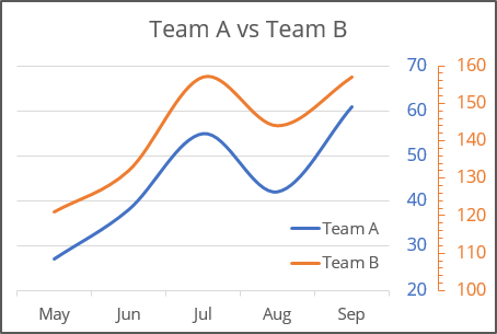
By default, Excel creates a chart with the primary horizontal axis at the bottom and with the primary vertical axis at the left side of the plot area (shown in blue in the example below). When you add the secondary vertical axis, Excel adds it at the right side (shown in orange):

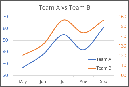
See also how to add the secondary horizontal axis and display both horizontal axes on the same side.

Add the secondary vertical axis

To add a secondary vertical axis, do the following:

   1.   Select the data series which you want to see using the secondary vertical axis.

   2.   Do one of the following:

• Right-click in the data series and choose Format Data Series... in the popup menu:
  

  On the Format Data Series pane, in the Series Options tab, select the Secondary Axis option instead of the Primary Axis:

  
• Right-click on the selection and choose Change Series Chart Type... in the popup menu:
  

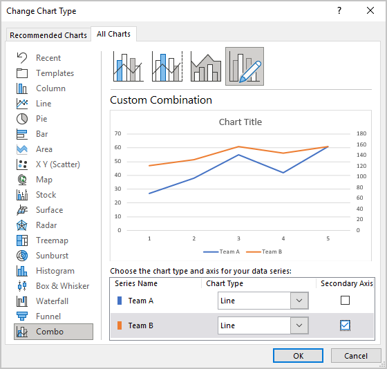
  In the Change Chart Type dialog box, select the Secondary Axis option for the appropriate data series:

Excel adds the secondary vertical axis for the selected data series:

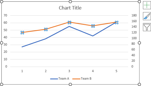
Display dual vertical axis on one side

   1.   Select the vertical axis that you want to move to the opposite side of the plot area, right-click on it and choose Format Axis... in the popup menu:

   2.   On the Format Axis pane, in the Axis Options tab, in the Labels section, choose the appropriate option from the Label Position drop-down list:

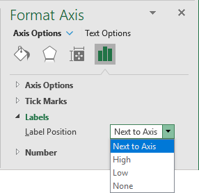
• Next to Axis (used by default) shows the primary vertical axis on the left side of the plot area, the secondary vertical axis on the right side of the plot area.
• High, shows the primary axis in the highest values of the data, on the right side (changes nothing for the secondary vertical axis):
  
• Low, shows the secondary axis in the lowest values of the data, on the left side (changes nothing for the primary vertical axis):
  
• None, hide labels for the axis. You still can select the axis, change its options, but can't see the labels.

See also this tip in French: Comment créer deux axes verticaux du même côté.