How to create Master and Scrolled Detail charts

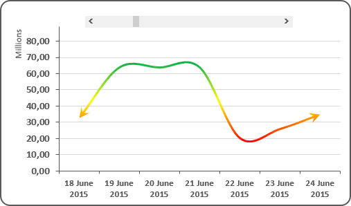
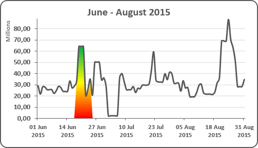
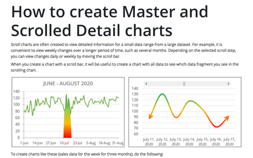
To create charts like these (sales data for the week for three months), do the following:

Step I: Create a chart with a scroll bar

See Creating a Scrolling chart).

Step II: Create a chart with total data

   1.   Select the data (in this example, B5:C96).

   2.   On the Insert tab, in the Charts group, click the Line button:

Choose the Line chart, delete the legend.

   3.   Move the chart so that it was placed under the chart with a scroll bar.

Step III: Add additional data

   1.   Add the next column to your data (in this example, C4:C95) and enter the following formula in the first cell:

= IF (AND (ROW (B5) >= $E$1 + 4, ROW (B5) - $E$1 < 7 + 4), C5, 0).

   2.   Copy this formula down to the other cells.

Step IV: Add a shaded box on the chart with a total data

   1.   Select the additional data (in this example, D5:D96), press Ctrl+C to copy the range. Select the bottom chart and press Ctrl+V to paste a new series to the chart.

   2.   Select the second data series and do one of the following:

• Under Chart Tools, on the Design tab, in the Type group, click the Change Chart Type button:
  
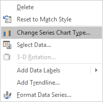
• Right-click on the selection and select Change Series Chart Type... in the popup menu:
  

   3.   In the Change Chart Type dialog box, choose the Area chart type for Series2:

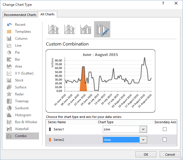
   4.   Click the area chart to select the second series. Under Chart Tools, on the Format tab, in the Shape Styles group, choose Shape Fill and select a color to make the shaded box:

See also this tip in French: Comment créer des graphiques de défilement principal et détaillés.