Glossy Gantt chart with a vertical line

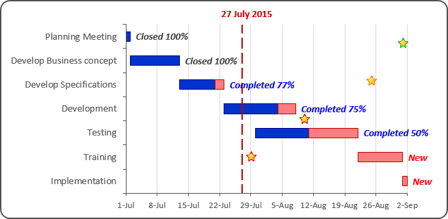
To add a vertical line in the current date, do the following:

   1.   Add the current date into your worksheet, select this cell, for example, F2:

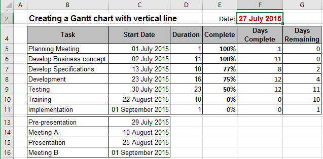
   2.   Do one of the following to add a new data series with cell F2:

   2.1.   Do one of the following:

• Under Chart Tools, on the Design tab, in the Data group, choose Select Data:
  
• Right-click in the chart area and choose Select Data... in the popup menu:
  

   2.2.   In the Select Data Source dialog box, click the Add button and in the Edit Series dialog box:

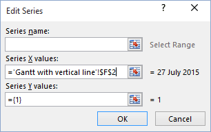
• In the Series X values box - the cells with dates ($F$2)
• In the Series Y values box - constant values (for example, {4}).

   2.3.   Click OK twice.

   2.4.   Change the secondary axis parameters, and then remove it.

   3.   Select new date series, then under Chart Tools, on the Design tab, in the Chart Layouts group, click the Add Chart Element icon and choose Error Bars list:

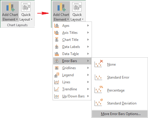
   4.   Select More Error Bars Options....

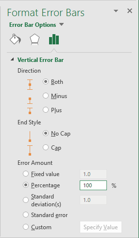
In the Format Error Bars dialog box, type parameters of the vertical line:

   5.   Make the new data series invisible. See also How to add a vertical line to the chart.

You can then make any other adjustments to get the look you desire.

See also this tip in French: Comment créer un diagramme de Gantt brillant avec une ligne verticale.