The Area chart for Investments

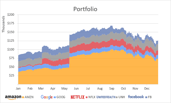
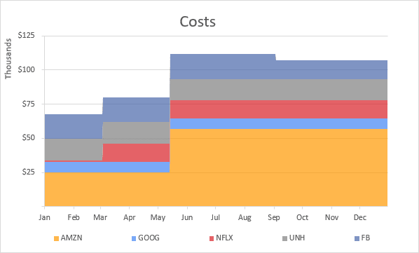
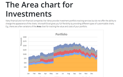
To create an Area chart like the ones above, do the following:

   1.   Write down the transaction data.

You can skip this step if you already have data for the chart.

   1.1.   Create or add to the workbook the buy/sell transactions for your stocks.

For example:

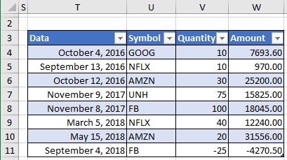
   1.2.   Add the stock price history to calculate the historical values of the portfolio positions.

Unfortunately, at the moment, Microsoft allows to download current stock prices, but not historical data.

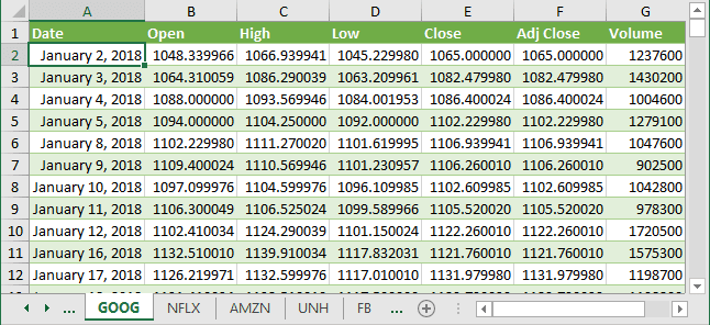
For this example, the historical data was downloaded from Yahoo Finance as a separate CSV files and uploaded to the workbook as separate sheets:

   1.3.   Create a portfolio positions valuation table:

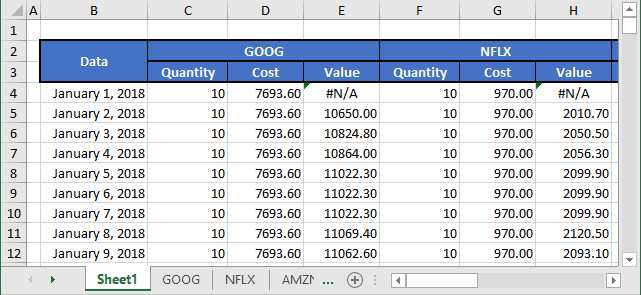
In this example, for every stock symbol was created three columns with the following formulas:

• Quantity:

  = SUMIFS (Transactions[Quantity], Transactions[Data], "<="&<data>, Transactions[Symbol], "="&<symbol>)

  where:

  • SUMIFS is a function to sum cells that meet multiple criteria:

    SUMIFS (<the range to be summed>, <the first range to evaluate>, <the criteria for the first range>, [<the second range>], [<the criteria for the second range>], ...)

  • Transactions is a table from p.1.1.,
  • <data> is an appropriate cell from column B,
  • <symbol> is a stock symbol from row 2.

  For the cell C4 this formula is:

  = SUMIFS (Transactions[Quantity], Transactions[Data], "<="&B4, Transactions[Symbol], "="&$C$2)

• Cost:

  = SUMIFS (Transactions[Amount], Transactions[Data], "<="&<data>, Transactions[Symbol], "="&<symbol>)

  For the cell D4 this formula is:

  = SUMIFS (Transactions[Amount], Transactions[Data], "<="&B4, Transactions[Symbol], "="&$C$2)

• Value:

  = <quantity> * INDIRECT (ADDRESS (MATCH (<quantity>, <data range>, 1), 5, 1, , <symbol>))

  where:

  • INDIRECT is a function that convert a reference assembled as text into a proper reference:

    INDIRECT (<a reference supplied as text>, [<the reference style>])

  • ADDRESS is a function that returns the address of a cell based on given row and column number:

    ADDRESS (<row number>, <column number>, [<the address type: absolute or relative>], [<the reference style>], [<sheet name>])

  • MATCH is a function used to locate the position of a lookup value in a row, column, or table:

    MATCH (<the value to lookup in the array>, <array>, [<match type>])

    With <match type> = 1 MATCH finds the largest value that is less than or equal to <the value to lookup in the array>.

  • <data range> is a table of historical data
  • <symbol> is a stock symbol from row 2.

  For the cell E4, this formula is:

  = C4 * INDIRECT (ADDRESS (MATCH (B4, GOOG!$A$1:$A$252, 1), 5, 1, , $C$2))

   2.   Select the data for the chart.

In this example, cells B4:B368 (dates), E4:E368 (GOOG), H4:H368 (NFLX), K4:K368 (AMZN), N4:N368 (UNH), Q4:Q368 (FB).

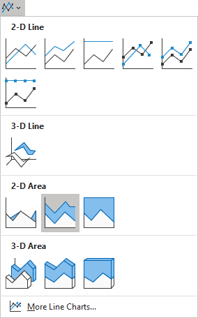
   3.   On the Insert tab, in the Charts group, click the Insert Line or Area Chart button:

In the Insert Line or Area Chart drop-down list, select Stacked Area:

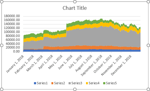
Excel creates a simple area chart:

   4.   To change the order of the data series and add the names of stocks, do the following:

   4.1.   Select data by one of the following ways:

• On the Chart Design tab, in the Data group, choose Select Data:
  
• Right-click in the chart area and choose Select Data... in the popup menu:
  

   4.2.   On the Select Data Source dialog box, for the Legend Entries (Series):

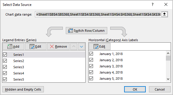
• Select the data series that you would like to rename and click the Edit button. In the Edit Series dialog box, type the name you prefer in the field Series name or select a cell with the appropriate name:
  
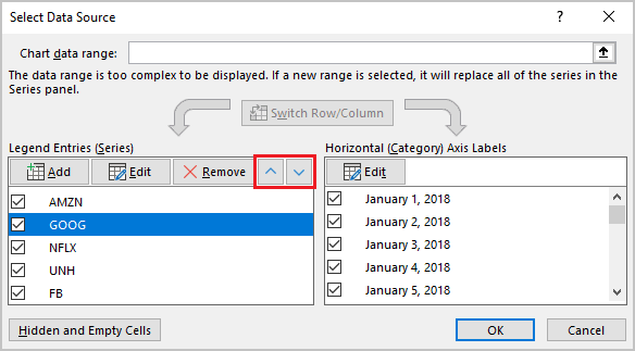
• Change the order for the data series by clicking the Move Up or Move Down buttons:

Make any other adjustments to get the look you like.