Logarithmic trend equation and forecast

Excel uses the least squares method to fit a trend line to the data points.
For a trend line, two sets of variables are required:
- an independent, predictor, or explanatory variable x (named as known_x's),
- a dependent or response variable y (named as known_y's).
Logarithmic trendline equation and formulas
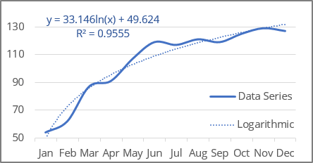
The logarithmic trendline is a curved line with the function:
y = a * ln (x) + b
where:
- a and b are the parameters of the function found by the least squares method (also named function coefficients or constants),
- ln is the natural logarithm function:
The LN () function returns the natural logarithm of a given number:
= LN (number)
where:
- number (required) is a number to take the natural logarithm of.
Note: Excel the logarithmic function approximation into the linear model fitting: the logarithmic function y = a * ln (x) + b is transformed into a linear function using a change of variables. After changing the variables to X = ln (x), the calculations become similar to the linear case Y = b * x + A:
Excel offers the following functions to calculate trendline parameters:
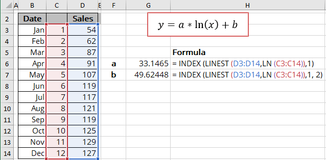
- a: = INDEX (LINEST (known_y's, LN (known_x's)), 1)
- b: = INDEX (LINEST (known_y's, LN (known_x's)), 1, 2)

The array function LINEST () calculates the linear trend that fits best the known data and then returns an array with statistics describing the trend line:
= LINEST (known_y's, [known_x's], [const], [stats])
where:
- known_y's (required) are dependent data values,
- known_x's (optional) are independent data values:
These variables cannot be omitted for the correct calculation for a logarithmic trend. In any case, you should provide the known_x's or array {1,2,3,...} that has the same size as known_y's,
- const (optional) is a Boolean value specifying whether to force the parameter b (intercept) to equal 0:
- If const is TRUE or omitted, the parameter b is calculated normally,
- If const is FALSE, the parameter b is set equal to 0.
- stats (optional) is a Boolean value specifying whether to return additional regression statistics:
- If stats is TRUE, the LINEST () function returns the additional regression statistics in the form of an array:

where:
Statistics Description a The parameter of the function b The intercept sea Standard error of the parameter a seb Standard error of the intercept R2 R-squared value sey Standard error of y estimate (also known as Standard Error of a regression) shows how big the prediction error is F F statistic (F-observed value) dr Degrees of freedom ssreg Regression sum of squares (also known as SSR) ssresid Residual sum of squares (also known as SSE) - If stats is FALSE or omitted, the function returns only the calculated parameters.
- If stats is TRUE, the LINEST () function returns the additional regression statistics in the form of an array:
Notes:
- If you have a version of Microsoft Excel other than Microsoft 365, functions that return arrays must be entered as array functions using Ctrl+Shift+Enter unless you can just press Enter.
- Because the LINEST () function returns an array of data, you can use the INDEX () function to display only the desired parameter(s) from the returned data array.
Calculating the logarithmic trendline values
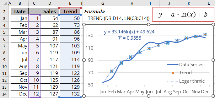
To calculate the logarithmic trendline values, Excel offers the array function TREND () (see the notes above about array functions) that returns values for a linear trend. To work with this function for logarithmic trends, just use LN (known_x's) instead of known_x's:
= TREND (known_y's, [known_x's], [new_x's], [const])
where:
- known_y's (required) are dependent data values,
- known_x's (optional) are independent data values:
These values cannot be omitted for the correct calculation for a logarithmic trend. In any case, you should provide the known_x's or array {1,2,3,...} that has the same size as known_y's,
- new_x's (optional) are the new x-values for which the TREND () function should calculate corresponding y-values:
- If you omit new_x's, it is assumed to be the same as known_x's.
- const (optional) is a Boolean value specifying whether to force the parameter b to be equal to 0:
- If const is TRUE or omitted, the parameter b is calculated normally,
- If const is FALSE, the parameter b is set equal to 0.

R-squared value
The R-squared value calculates to determine how well a trendline fits the data (in Excel, R2). The R-squared value can vary from 0 to 1: the nearer R2 is to 1, the better the trendline fits the data.
The R-squared value can be displayed on the chart (see how to turn on the R-squared value). You can easily calculate that value using one of the following methods:
- Use the LINEST () function to return the first statistics of the third line in the statistics array:
= INDEX (LINEST (known_y's, LN (known_x's), , TRUE), 3, 1):

- Use the RSQ () function that returns the R-squared value of two data sets:
= RSQ (array1, array2)
where array1 and array2 (both are required) are two data sets:

Forecast using the logarithmic trendline
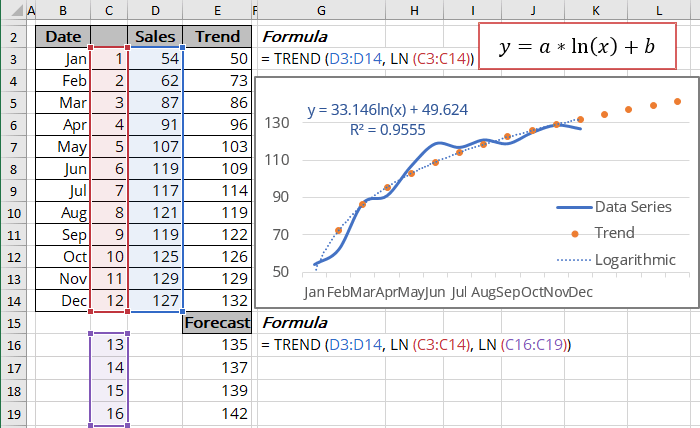
Using the TREND () function, you can calculate the predicted values y for the new_x's (don't forget to add the natural logarithm function for the new_x's):

To calculate forecasts, Excel offers another array function (see the notes above about array functions) - FORECAST.LINEAR () that returns the same results (at least for our experiments):
= FORECAST.LINEAR (x, known_y's, known_x's)
where:
- x (required) can be one value or data range of new x-values for the FORECAST.LINEAR () function should calculate corresponding y-values,
- known_y's (required) are dependent data values,
- known_x's (required) are independent data values.
Note: Don't forget to add the natural logarithm function for known_x's and x. The function should look like this:
= FORECAST.LINEAR (LN (x), known_y's, LN (known_x's)).


