Linear trend equation and forecast

Trendlines can be different (see trendlines types in Excel), but the most common and simplest one is the linear trend line:

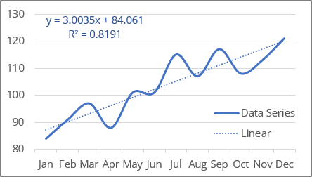
Excel uses the least squares method to fit a linear line estimator for the data points.

For a trend line, two sets of variables are required:

• an independent, predictor, or explanatory variable x (named as known_x's),
• a dependent or response variable y (named as known_y's).

Linear trendline equation and formulas

The linear trendline is a straight line with the function:

   y = ax + b

where a and b are calculated parameters of the linear function (also named as coefficients or constants):

• a is a slope of a trendline (steady rate - the average change in the dependent variable y for a one unit increase in independent variable x),
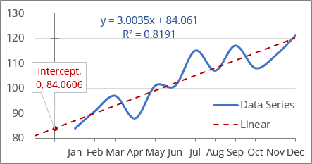
• b is an intercept, the value of dependent variable y when the independent variable x = 0. On a chart, it's the point where the trendline crosses the y axis:

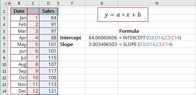
Excel offers the following functions to calculate trendline parameters:

To calculate the parameter b (intercept)

The INTERCEPT () function calculates the y value at which the linear trendline crosses the y-axis. In other words, using the known_x's and known_y's data, it returns the value y of the function for x = 0:

= INTERCEPT (known_y's, known_x's)

where:

• known_y's (required) are dependent data values - a range or array of numeric values,
• known_x's (required) are independent data values (see an example below) - a range or array of numeric values.

To calculate the parameter a (slope)

The SLOPE () function returns the slope (the parameter a) of a linear regression line based on known_y's and known_x's data:

= SLOPE (known_y's, known_x's)

where:

• known_y's (required) are dependent data values - a range or array of numeric values,
• known_x's (required) are independent data values (see an example below) - a range or array of numeric values.

Notes:

1. If there is only one value in known_y's or known_x's, the INTERCEPT () and SLOPE () functions will return #DIV/0!
2. If the count of known_y's is different from known_x's, the INTERCEPT () and SLOPE () functions returns #N/A.

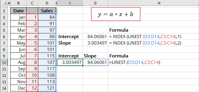
You can also use the array function LINEST () that calculates the linear trend that fits best the known data and then returns an array with statistics describing the trend line:

= LINEST (known_y's, [known_x's], [const], [stats])

where:

• known_y's (required) are dependent data values,
• known_x's (optional) are independent data values. If known_x's is omitted, it is assumed to be the array {1,2,3,...} that has the same size as known_y's,
• const (optional) is a Boolean value specifying whether to force the parameter b (intercept) to equal 0:
  • If const is TRUE or omitted, the intercept is calculated normally,
  • If const is FALSE, the intercept is set equal to 0.
• stats (optional) is a Boolean value specifying whether to return additional regression statistics:
  • If stats is TRUE, the LINEST () function returns the additional regression statistics in the form of an array:
    

    where:

    Statistics	Description
    a	The slope
    b	The intercept
    sea	Standard error of the slope
    seb	Standard error of the intercept
    R2	R-squared value
    sey	Standard error of y estimate (also known as Standard Error of a regression) shows how big the prediction error is
    F	F statistic (F-observed value)
    dr	Degrees of freedom
    ssreg	Regression sum of squares (also known as SSR)
    ssresid	Residual sum of squares (also known as SSE)

  • If stats is FALSE or omitted, the LINEST () function returns only the slope and the intercept.

Notes:

1. If you have a version of Microsoft Excel other than Microsoft 365, functions that return arrays must be entered as array functions using Ctrl+Shift+Enter unless you can just press Enter.
2. Because the LINEST () function returns an array of data, you can use the INDEX () function to display only the desired parameter(s) from the returned data array:

Calculating the linear trendline values

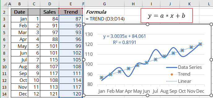
To calculate the linear trendline values, Excel offers the array function TREND () (see the notes above about array functions) that returns values along a linear trend:

= TREND (known_y's, [known_x's], [new_x's], [const])

where:

• known_y's (required) are dependent data values,
• known_x's (optional) are independent data values. If known_x's is omitted, it is assumed to be the array {1,2,3,...} that has the same size as known_y's,
• new_x's (optional) are the new x-values for which the TREND () function should calculate corresponding y-values:
  • If you omit new_x's, it is assumed to be the same as known_x's,
  • If you omit both known_x's and new_x's, they are assumed to be the array {1,2,3,...} that is the same size as known_y's.
• const (optional) is a boolean value specifying whether to force the parameter b (intercept) to equal 0:
  • If const is TRUE or omitted, the intercept is calculated normally,
  • If const is FALSE, the intercept is set equal to 0.

R-squared value

The R-squared value (in Excel, R²) is calculated to determine how well a trendline fits the data. The R-squared value can vary from 0 to 1: the nearer R² is to 1, the better the trendline fits the data.

The R-squared value can be displayed on the chart (see how to turn on the R-squared value). You can easily calculate that value using one of the methods:

• Use the LINEST () function to return the first item from the third line of the statistics array:

  = INDEX (LINEST (known_y's, known_x's, , TRUE), 3, 1):

  
• Use the RSQ () function that returns the R-squared value of two data sets:

  = RSQ (array1, array2)

  where array1 and array2 (both are required) are two data sets:

  

Forecast using the linear trendline

Using the TREND () function, you can calculate the predicted values y for the new_x's:

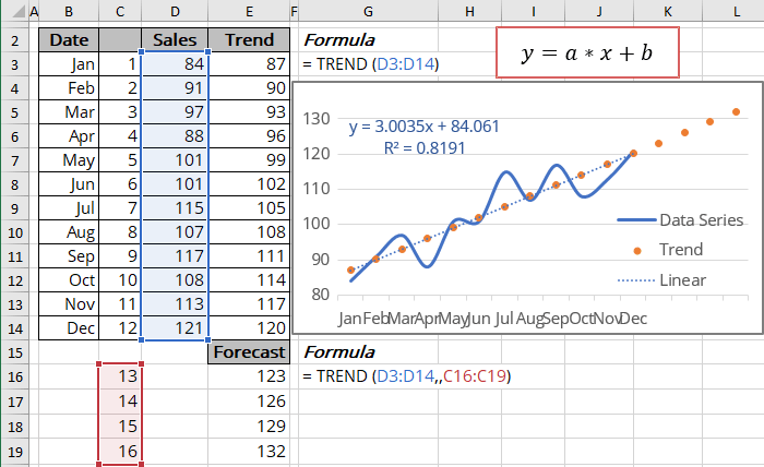
To calculate forecasts, Excel offers another array function (see the notes above about array functions) - FORECAST.LINEAR () that returns the same results (at least for our experiments):

= FORECAST.LINEAR (x, known_y's, known_x's)

where:

• x (required) can be one value or data range of new x-values for the FORECAST.LINEAR () function should calculate corresponding y-values,
• known_y's (required) are dependent data values,
• known_x's (required) are independent data values.