How to create re-sorting chart in Excel

One of the most common tips when creating comparison charts without favorites is to sort the data by some key parameter.

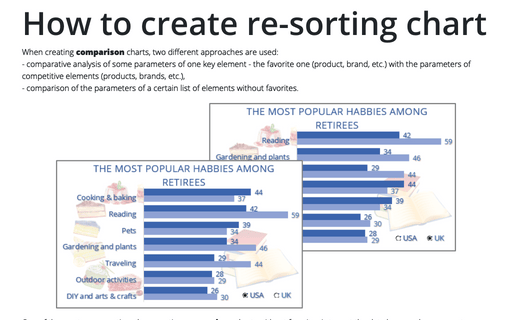
In Excel, you can easily create a chart in which you can switch the option by which to sort the proposed elements of the comparison list:

To create an interactive chart, add one of the controls: Option Buttons (radio buttons), Check Boxes, or Combo Box (drop-down list). See other techniques for creating interactive charts.

To create a re-ordering interactive chart with option buttons, do the following:

   1.   Prepare the data that will be shown in the chart

Add the new data to select one of the parameters.

For example, enter in the cell F2 the number 1:

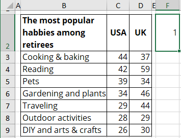
   1.2.   To the next cells, add the following formula:

The CHOOSE (<index>, <first item>, <second item> ...) function returns the value from the list (<first item>, <second item>, etc.) specified by the first parameter <index>.

In this example:

= SORTBY (B2:D9, CHOOSE ($F$2, C3:C9, D3:D9))

So, you will see the sorted array by the chosen index:

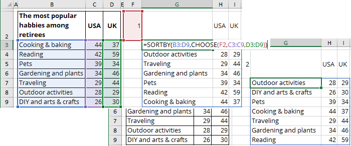
Note: You can define names instead of using this formula on the spreadsheet.

   2.   Create a chart

Create a simple bar chart or any other chart you prefer (see more about different charts in Excel) using the calculated data (or defined names).

For example:

   3.   Add the option buttons to the chart

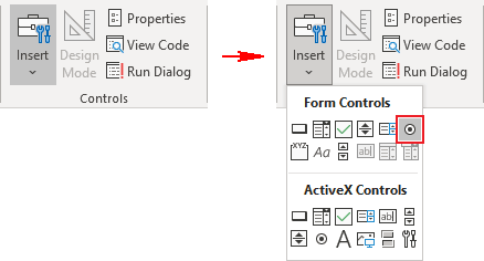
   3.1.   On the Developer tab (see Show the Developer tab), in the Controls group, click the Insert drop-down list and then choose Option Button (Form Controls):

Note: You can also add to the Quick Access Toolbar (see how to add commands to the Quick Access Toolbar):

• The entire Insert controls dropdown list:
  
• The Option Button control.

Add as many option buttons as the number of series selected by these option buttons and place them where you want.

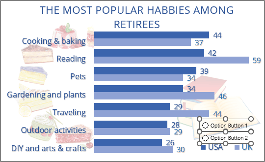
In this example, just two option buttons were used:

   3.2.   Format Option buttons:

To create a more effective view, place the Option buttons under Legend points and remove buttons names:

   3.2.1.   Double-click on every Option button and change the label - remove it.

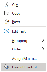
   3.2.2.   Right-click on each Option button and choose Format Control... in the popup menu:

   3.2.3.   In the Format Control dialog box, on the Control tab, choose the appropriate cell in the Cell link field (in this example, F2):

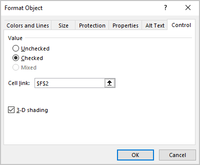
The trick to using Option buttons is to assign the same cell to all the Option buttons in a particular group. Initially, the cell value is assigned to the first element of the option group. Next, all added Option buttons will automatically use and change the value of this cell.

Note: To change the sizes of the control or move it, right-click on the control to select it, then click it again to close the popup menu.