How to create Budget Template that works for you

A budget matches your known or expected income to your necessary monthly expenses. Then you decide how to distribute any remaining cash - your discretionary income. Set aside enough money from each paycheck to pay the bills and save some for the "rainy day" if possible. For many people, that defines the scope of their budgeting - spend what you need, save what you can.

Moving in the right direction is typically easy, but it does not necessarily get you where you want to go. A little overspending here and there, unexpected expenses, and the dream gets a little further away. Meanwhile, the word budget immediately evokes unpleasant images of prison. A restrictive set of rules telling you what you can and cannot do.

Budgets do not have to be thought of that way - think of them as spending plans instead. Although it sounds like wordplay, budgets and spending plans are different, if only because of the psychological reaction they evoke. Where budgets represent restriction, spending plans represent freedom because you make conscious decisions about spending or saving your money:

• You can choose to pay off your credit card or car to get out of debt faster.
• You can choose to put that money toward a vacation, a new washing machine, or a fancy meal at a restaurant with your significant other.
• You can choose to buy shares in a mutual fund, open a Roth IRA or fund a college savings account for your child.

You can do whatever you want with your money because you are in charge.

Create budget template

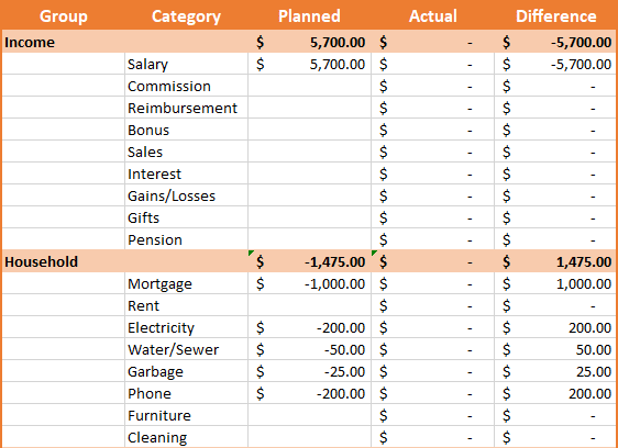
You will need a broad set of categories to create a spending plan. However, creating and analyzing highly detailed budget plans with numerous revenue and expense types takes too much time and effort. Therefore, it is necessary to combine categories into groups from the very beginning in the Income & Expenses spreadsheet:

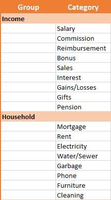
Having a grouping of your financial assets in the Accounts spreadsheet is also a good idea:

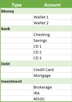
Later, it will be helpful for the accounting and estimation of your net worth.

To create a monthly budget, you need three columns:

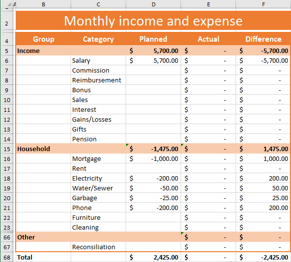
• Planned - estimates of how much you expect to earn and spend in each income/expense category that applies to your life. For salary, car payment, or rent, this will be easy. For bonuses, food, and entertainment, it is more of a guess. Some income and expenses may be unexpected and difficult to plan for. Ideally, the planned amount for the group should equal the sum of all categories.

  For example, for the Income group: = SUM (D6:D14).

  Also, you can simply use a planned amount for the entire group.

• Actual - contains amounts for each income and expense category for the current month.
• Difference - shows the difference between your plans and reality.

In addition, you will need the Total row that adds up the amounts in each of the columns. Hierarchical budget spreadsheets are great for planning and analysis but difficult to create because simply summing the entire column will not give a correct total. You need to sum amounts either for groups or for categories. The following formula will be used in the Total row:

= SUMIF ($B5:$B67, "<>", D5:D67)

For the child categories, the Group column cells are blank. Thus, the $B5:$B67, "<>" criterion is FALSE for the categories and TRUE for the groups. Therefore, only group amounts from the range D5:D67 are selected for summing - that is exactly what is required.

Since the Total row adds up all revenues, expenses, and investments, the balances in the Total row give you simple clues for planning and execution:

• If the balance is negative in the Planned column, you need to rethink some of your anticipated expenses. Otherwise, you will be in debt for the month, or you will reduce your savings.
• If the balance in the Actual column is negative, you went into debt for the month and need to take a hard look at your spending to see where you went too far off track. You will likely have to postpone other planned expenses in other categories. You do not have to worry about the negative balance in the Actual column before receiving your paycheck.
• If the balance in the Actual column is positive, you need to put that money somewhere. Spending in categories important to you, using unspent income to pay down any credit card debt, car loan, or mortgage, or putting into additional savings at the end of the month will ultimately make your balance $0.

This budget template is sufficient for budgeting with a certain level of discipline. However, we will build a proper tracking table with automatic income and expense accounting.

Create tracking spreadsheet

Analyzing how much you earn and how you spend should not be like a detective trying to reconstruct a crime scene. Who needs to keep records in the age of online banking? Recent pay stubs, electronic bills, credit card statements, etc., make record-keeping obsolete. Avoid jumping to conclusions; in fact, all online services are designed to make the truth less obvious — multiple bank accounts, extra fees here and there, delays in settlement, and cash. Purchases made with cash are the most difficult to track because they leave no trace on your bank statements except for withdrawals.

Paper, pencil, and a calculator worked just fine to keep track of your income and expenses in the 20th century. Housing, clothing, food, and transportation were all you needed to keep track of. Nowadays, you have multiple subscriptions and financial obligations such as credit cards, loans, and insurance payments, and old tools no longer work.

Today we have Excel, and we just need to use it properly. An Office 365 subscription is probably one of the best ways to put your money to work.

To create the Income and Expense tracker, do the following:

Create Tracking table

   1.   Create a new spreadsheet and rename it to Tracking.

   2.   Type the column names in the row and select a few extra rows:

   3.   On the Insert tab, in the Tables group, click the Table button:

   4.   In the Create Table dialog box:

• Ensure that in the Where is the data for your table? field is selected the correct data range,
• Select the My table has headers check box,
• Click the OK button:

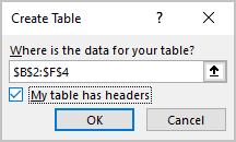
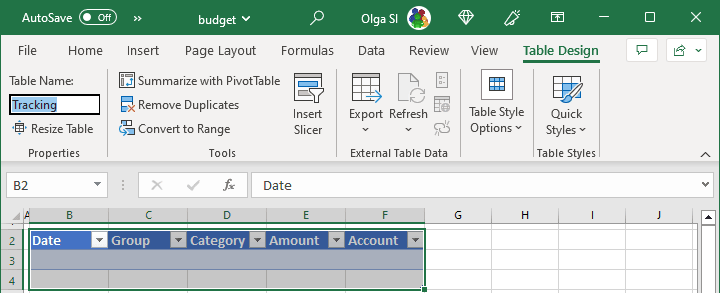
Excel will create a new table definition and displays the Table Design tab:

   5.   Type Tracking in the Table Name field on the Table Design tab:

   6.   Choose a proper cell format for the Date and Amount columns.

Now comes the hardest part - creating drop-down lists for the Group, Category, and Account columns.

Create drop-down lists

Creating drop-down lists is done in three steps:

• Create named ranges for accounts and categories.
• Create simple drop-down lists for groups and accounts.
• Create dependent drop-down lists for categories.

Create named ranges for accounts and categories

   1.   On the Formulas tab, click the Define Name button:

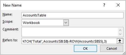
   2.   In the New Name dialog box:

• In the Name field, type AccountsTable,
• In the Refers to field, enter the following formula:

  = OFFSET (Accounts!$B$5, 0, 0, MATCH ("Total", Accounts!$B:$B) - ROW (Accounts!$B$5), 3)

• Click the OK button:

Repeat the steps above to create the CategoriesTable with the following formula:

= OFFSET ('Income & Expense'!$B$5, 0, 0, MATCH ("Total", 'Income & Expense'!$B:$B) - ROW ('Income & Expense'!$B$5), 5)

The point is to get a handy reference to the data range below the table header and above the Total row:

• OFFSET ('Income & Expense'!$B$5, 0, 0, ...) returns a range of the specified height and width (3 for the accounts table / 5 for the categories table) starting at the first cell of the categories table.
• MATCH ("Total", 'Income & Expense'!$B:$B) finds the row number of the Total row.
• MATCH (...) - ROW ('Income & Expense'!$B$5) finds the height of the data range.

Create simple drop-down lists for groups and accounts

Before creating drop-down lists for the Groups and Accounts columns, select the data from the Categories and Accounts tables and create the named ranges:

• CategoriesList with the following formula:

  = TOCOL (OFFSET (CategoriesTable, 0, 0, , 1), 1)

  where

  • OFFSET (...) returns the first column of the Categories table;
  • TOCOL (..., 1) returns a column of non-blank values.
• GroupsList with the following formula:

  = TOCOL (OFFSET (AccountsTable, 0, 1, , 1), 1)

  where

  • OFFSET (...) returns the first column of the Accounts table;
  • TOCOL (..., 1) returns a column of non-blank values.

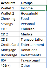
Drop-down lists in Excel do not accept data in an array format. You must provide a list of values or a range of cells. To do this, simply add the Data Lists worksheet and type =AccountList and =GroupList, and array references automatically spill over the column:

To create drop-down lists for the Groups and Accounts columns, do the following:

   1.   Select the data cells in the column.

   2.   On the Data tab, in the Data Tools group, click the Data Validation button:

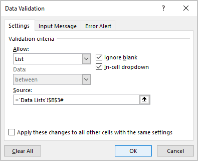
   3.   In the Data Validation dialog box:

• From the Allow drop-down list, select the List option,
• In the Source field, enter the hash reference ='Data Lists'!$B$3# to the first cell of the spill range:

Create dependent drop-down lists for categories

The Group cell of the Tracking table determines the data in the Category cell drop-down list. To do this, create another named range called CategoryList with the following formula:

= OFFSET (CategoriesTable, MATCH (Tracking[@Group], OFFSET (CategoriesTable, 0, 0, , 1), 0), 1, MATCH (TRUE, ISBLANK (OFFSET (CategoriesTable, MATCH (Tracking[@Group], OFFSET (CategoriesTable, 0, 0, , 1), 0), 1, , 1)), 0) - 1, 1)

which can be represented as follows

= OFFSET (CategoriesTable, #GroupStart#, 1, #GroupHeight#, 1)

where

• #GroupStart# is MATCH (Tracking[@Group], CategoryColumn, 0) finds the starting row of the required fragment;
• #CategoryColumn# is OFFSET (CategoriesTable, 0, 0, , 1) returns the category column data;
• #GroupHeight# is MATCH (TRUE, ISBLANK (#CategoriesBelow#, 0) - 1 finds the height of the required fragment. The height is an index of the first blank cell after the group starting row;
• #CategoriesBelow# is OFFSET (CategoriesTable, #GroupStart#, 1, , 1)).

If you wish, you can create the named ranges for CategoryColumn, GroupStart, CategoriesBelow, and GroupHeight.

To create the dependent drop-down list for the Category column, do the following:

   1.   Select the data cells in the column.

   2.   On the Data tab, in the Data Tools group, click the Data Validation button.

   3.   In the Data Validation dialog box:

• From the Allow drop-down list, select the List option.
• In the Source field, enter the formula =CategoryList.

Create slicers

Slicers are not required to track income and expenses. However, they make it easier to filter tables. Adding slicers for the Group, Category, and Account columns is particularly useful.

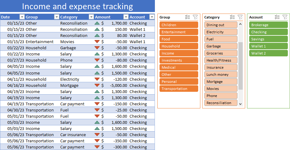
To add slicers, do the following:

   1.   Select the Tracking table cell.

   2.   On the Table Design tab, in the Tools group, click the Insert Slicer button:

   3.   In the Insert Slicer dialog box, select the Group, Category, and Account checkboxes, then click the OK button:

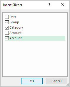
For the Date column, configure the filter in the table's header. The most convenient filter is to limit the table data to the current month and empty cells.

Update budget spreadsheet

The Tracking spreadsheet puts your budget on autopilot and lets you fly. You can update the Actual column automatically by summing the Tracking table amounts for the group/category in the current month:

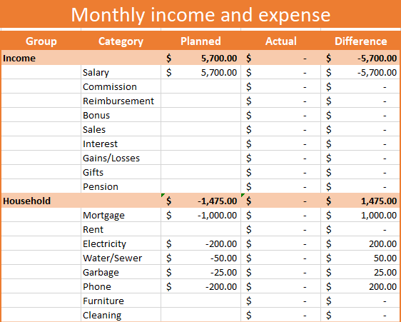
The SUMIF magic used above does not apply here, but there is SUMPRODUCT magic. Put the following formula into the group rows of the Actual column:

= SUMPRODUCT (Tracking[Amount], INT (Tracking[Group] = B5), INT (MONTH (Tracking[Date]) = MONTH (TODAY ())))

and the following formula into the category rows:

= SUMPRODUCT (Tracking[Amount], INT (Tracking[Category] = C6), INT (MONTH (Tracking[Date]) = MONTH (TODAY ())))

where

• Tracking[Group] = B5 returns an array of TRUE/FALSE for groups, and INT converts it to the array of 1/0 elements.
• Tracking[Category] = C6 returns an array of TRUE/FALSE for categories, and INT converts it to the array of 1/0 elements.
• MONTH (Tracking[Date]) = MONTH (TODAY ()) returns an array of TRUE/FALSE for dates in the current month, and INT converts it to the array of 1/0 elements.
• SUMPRODUCT finds a sum of Tracking[Amount] * ... * INT (MONTH (Tracking[Date]) = MONTH (TODAY ())) products, i.e., sums amounts for the specified group/category for the current month.

Update accounts spreadsheet

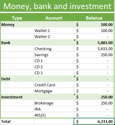
Update the accounts table with the Balance column to get the full picture of your net worth:

= SUMIF (Tracking[Account], C6, Tracking[Amount])

and add the Total row:

= SUMIF ($B5:$B20, "<>", D5:D20)

Conclusion

Although your expenses change each month and your income covers your needs and wants, certain life events require you to take a much broader look at your plan and adjust it to meet the changing needs of your income:

• Marriage or divorce.
• Salary decreases or layoffs.
• Birth or adoption of a child.
• Car or home purchases.
• Temporal disability.
• Retirement.

These events require you to include in your personal budget or spending plan an amount of money that you automatically take out of your income each month and put into a savings, money market, or retirement account.

Take control of your life with this budget template!