How to create a Scrolling chart
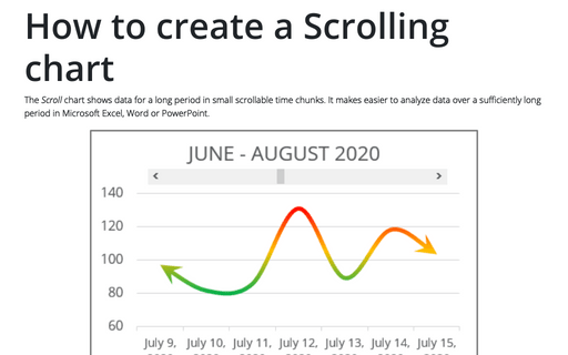
The Scroll chart displays some contiguous range of data from a large dataset. Using the provided Control tools, it is possible to add a scroll bar to the chart area and view the desired data range:

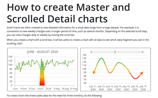
See also Creating Master and Scrolled Detail Charts.
To create a chart like the one above (sales data for the week for three months), do the following:
Step I: Create a chart
1. Select the data (in this example, B2:C95).
Note: You can select any data range and click Ctrl+Shift+Space to select the data range (see How to select row and column by keyboard and How to select a large data range in one click in Excel for more details).
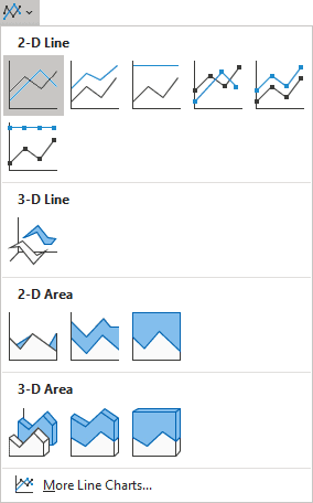
2. On the Insert tab, in the Charts group, click the Insert Line or Area Chart button:

From the Insert Line or Area Chart, choose Line:

Excel creates a simple line chart:

Step II: Create additional data
1. Enter 1 in any cell (in this example, E2) - this number will be used for scrolling (the scrolling cell).
2. On the Formulas tab, in the Defined Names group, click the Name Manager button:

3. In the Name Manager dialog box, click the New... button:

4. In the New Name dialog box:

- Type the name (for example, Dates) in the Name field.
- In the Refers To field, enter the formula:
= OFFSET (Scroll!$B$2, Scroll!$E$2, 0, 7).
The OFFSET () function returns a cell or range of cells that is a specified number of rows and columns from a cell or range of cells: = OFFSET (<reference>, <row>, <column>, [height], [width])
So, in this example, the formula says to start from cell B2 of the Scroll sheet, move down the number of rows defined in in cell E2 (scrolling cell), and then take a range of 7 rows (one week) by the first column.
- Click OK to accept the name.
5. In the Name Manager dialog box, click the New... button to add another name (for example, Sales) with the following formula in the Refers To box:
= OFFSET (Scroll!$B$2, Scroll!$E$2, 1, 7).
The only change is that in the third argument, you move right one column to grab data from column C.
6. Click the line series in the chart. Wait for the SERIES formula to appear in the formula bar. Edit the formula so that it looks like this:
= SERIES (Scroll!$B$2, Scroll!Dates, Scroll!Sales, 1):

Test the chart. Enter a new number between 1 and the maximum valid value in the cell E2. The chart should change.
Maximum valid value = length of the data range - length of visible data + 1.
For this example, the last valid value is:
93 (number of days in the data range B2:C95 without headings) - 7 (one week) + 1 = 87.
Step III: Add a scroll bar
On the Developer tab (if you don't have the Developer tab available in the ribbon, see Show the Developer tab), in the Controls group, click the Insert button and then choose the Scroll Bar icon:

Note: You can also add to the Quick Access Toolbar (see Adding commands to the Quick Access Toolbar):
- The entire Insert controls dropdown list:

- The Scroll Bar control:

Step IV: Customize the scroll bar
1. Right-click the scroll bar and choose Format Control... in the popup menu:

2. In the Format Control dialog box, on the Control tab:

- Change Minimum value to 1
- Change Maximum value to your maximum valid value
- Set Incremental Change to 1 (or to 7 to scroll between weeks instead of days)
- In the Cell link field, choose a scrolling cell with the scroll point (in this example, E2)
- Click OK. Click outside the scrollbar to deselect it.
Notes:
- To test the scrollbar, drag the slider. The value in cell E2 should change; the top chart should also change.
- To change the sizes of the scroll bar or move it, right-click it to select the scroll bar, then click it again to close the popup menu.
- Excel works quite correctly if you scroll through the chart step by step. However, Excel may lose custom chart settings if you jump a few steps forward or backward using the scroll bar.
To avoid switching your chart to the default chart settings, you can change the default colors that Excel uses for chart series.
See also this tip in French: Comment créer un graphique de défilement.

