Creating automatically extended plot ranges

You can force Excel to update a new or existing chart automatically when you add new data. To do so, follow the next steps:

Prepare data

   1.   On the Formulas tab, in the Defined Names group, click Define Name:

Define data for the horizontal (Category) axis

   2.   In the New Name dialog box:

• In the Name field, enter Data,
• In the Refers to field, enter this formula:

  = OFFSET (<Sheet name>!<start cell>, 0, 0, COUNTA (<Sheet name>!<Column name>:<Column name>) - 1)

  

  The OFFSET () function returns a cell or range of cells that is a specified number of rows and columns from a cell or range of cells:

  = OFFSET (<reference>, <row>, <column>, [height], [width])

  Note: See below how to use the range from row instead of column.

• Click the OK button to close the New name dialog box.

See more about creating and using named ranges.

Notice that the OFFSET () function refers to the first data point (cell B3) and uses the COUNTA () function to get the number of data points in the column.

Define data for the vertical (Value) axis

   3.   Define a new data range in the New Name dialog box:

Modify a chart

   4.   Select the chart and do one of the following:

• On the Chart Design tab, in the Data group, choose Select Data:
  
• Right-click in the chart area and choose Select Data... in the popup menu:
  

   5.   On the Select Data Source dialog box, change the range of data series and axis with the names that you defined in Steps 2 and 3:

   5.1.   Under Legend Entries (Series):

• Select the data series that should be updated automatically and click the Edit button.
• In the Edit Series dialog box, type the previously defined data range name for the data series (step 3).

  For this example:

  

  Series values: <Excel-file name>!Sales or <Excel-file name>!Sales

  Note: If you type the sheet name, Excel automatically changes it to the file name:

  

   5.2.   Under Horizontal (Category) Axis Labels:

• Click the Edit button.
• In the Axis Labels dialog box, type the previously defined data range name for the axis (step 2).

  For this example:

  

  Axis label range: <Excel-file name>!Data

  Note: If you type the sheet name, Excel automatically changes it to the file name:

  

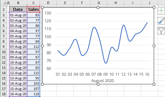
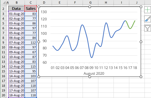
After you perform these steps, when you add data to columns B and C, the chart updates automatically to show the new data (see at the top of this tip). To use this technique for your own data, ensure:

• that the first argument for the OFFSET () function refers to the first data point,
• that the argument for COUNTA () refers to the entire column of data.

Also, if the columns used for the data contain any other entries, COUNTA () will return an incorrect value.

Notes:

1. If the axis doesn't change automatically, check:
   • The formulas in the chart,
   • The defined minimum and maximum values for the axis - Excel can't change custom values:
     

   To allow Excel to change axis ranges, click the Reset button.

2. The COUNTA () function was used in this example to avoid counting blank cells.

   Cells with formulas or filled with irrelevant information, such as comments, will also be counted as non-empty. Because of this, we used the COUNTA () - 1 to exclude the cell with column name (in this example: Data and Sales).

   In this case, replacing the COUNTA () function with another one is necessary. For example:

   • COUNT () counts only cells with numbers, but it also has issues depending on the data. In some cases, the COUNT () function can calculate formula results you don't want to show in the chart.
   • COUNTIF () can count cells that contain numbers. For example:

     COUNTIF (<data range>, ">0").

3. If you need to use the data from rows instead of columns, change the formula code to:

   = OFFSET (<Sheet name>!<start cell>, 0, 0, 1, COUNTA (<Sheet name>!<Row name>:<Row name>) - 1):

   
   

See also this tip in French: Comment créer les graphiques avec les plages de tracé étendues automatiquement.