Creating automatically extended plot ranges

To force Excel to update your chart automatically when you add new data, follow these steps:

   1.   On the Formulas tab, in the Defined Names group, click Define Name:

   2.   In the New Name dialog box, in the Name field, enter Date, and in the Refers to field, enter this formula:

=OFFSET(<Sheet name>!<start cell>,0,0,COUNTA(<Sheet name>!<Column name>:<Column name>) - 1)

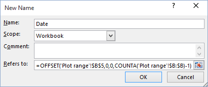
   3.   Click OK. Notice that the OFFSET function refers to the first data point (cell B5) and uses the COUNTA function to get the number of data points in the column.

   4.   Type Sales in the Name field, and in the Refers To field enter the same formula only for Sales data:

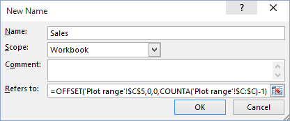
   5.   Click OK to close the dialog box.

   6.   Create the chart.

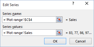
   7.   Change the range of data series and axis with the names that you defined in Steps 2 and 4:

• Series values: <Excel-file name>!Sales

• Axis label range: <Excel-file name>!Date

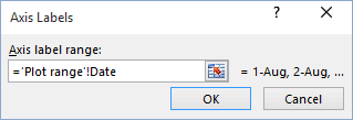
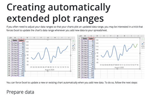
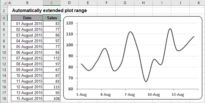
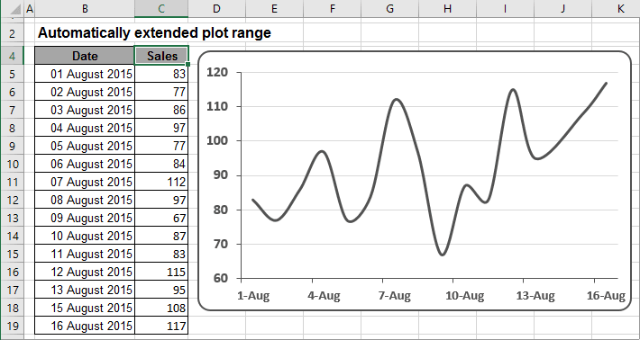
After you perform these steps, when you add data to columns B and C, the chart updates automatically to show the new data (see on the top of this screen). To use this technique for your own data, make sure that the first argument for the OFFSET function refers to the first data point, and that the argument for COUNTA refers to the entire column of data. Also, if the columns used for the data contain any other entries, COUNTA will return an incorrect value.

See also this tip in French: Comment créer les graphiques avec les plages de tracé étendues automatiquement.