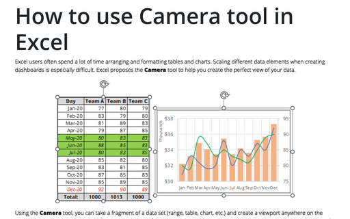
How to use Camera tool in Excel

The Camera tool isn't included in the standard ribbons of Microsoft Excel 2016, but you can add it:

• To your own Ribbon or group (see Creating your own menu):
  
• To the Quick Access Toolbar (see Adding commands to the Quick Access Toolbar):
  

To create a new picture from your table or chart, do the following:

   1.   Select data that you want to show in the screenshot.

For example:

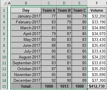
   2.   Click on the Camera button.

   3.   Select the area where you want to paste the screenshot.

   4.   Position the screenshot where you want:

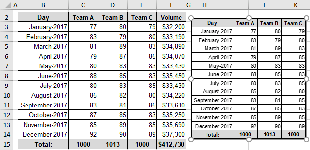
You can change the screenshot parameters and positioning it when you prefer. When you change something in the source table, it will be changed in the screenshot too:

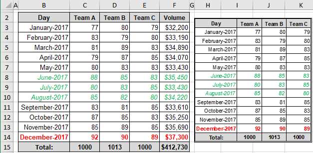
Note: We strongly recommend to avoid using the Camera Tool for charts. Sure, it works, but Excel still generate errors when we try to change anything in the source chart.

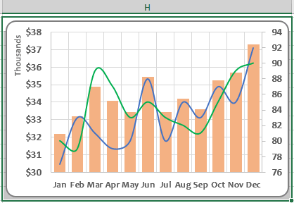
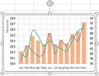
To create a screenshot from the chart, you need to position it in some cells and create a screenshot from cells. You can change width of gridlines or even turn off gridlines in Excel.

For example:

- The selected cells:

- The screenshot:

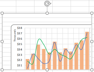
Be careful, if you change the position of that chart, the screenshot will be changed regarding to the cells data, not to the chart!

See also this tip in French: Comment utiliser l'outil Appareil photo dans Excel.