Excel 3-D Pie charts

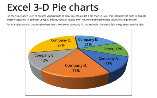
If you want to create a pie chart that shows your company (in this example - Company A) in the greatest positive light:

Do the following:

   1.   Select the data range (in this example, B5:C10).

   2.   On the Insert tab, in the Charts group, choose the Pie button:

Choose 3-D Pie.

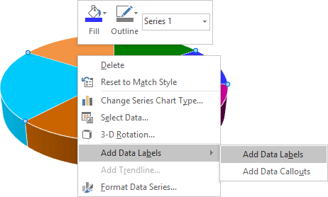
   3.   Right-click in the chart area, then select Add Data Labels and click Add Data Labels in the popup menu:

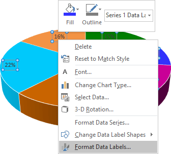
   4.   Click in one of the labels to select all of them, then right-click and select Format Data Labels... in the popup menu:

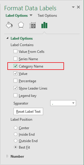
   5.   On the Format Data Labels pane, in the Label Options tab, select the Category Name checkbox:

   6.   Right-click in the data series and select Format Data Series... in the popup menu:

   7.   On the Format Data Series pane:

• In the Series Options section:
  • In the Angle of first slice field, move the sliding handle to the rotation degree that you want, or type a number between 0 and 360 degrees. The default setting is 0 degrees.
  • In the Pie Explosion field, move the sliding handle to the percentage of the explosion that you want, or type a percentage between 0 and 400 in the text box. The default setting is 0%.
  
• In the Effects section, in the 3-D Format group, make changes you want.

You can then make any other adjustments to get the look you desire.

See also this tip in French: Graphiques à secteurs 3-D.