Speedometer chart

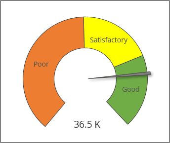
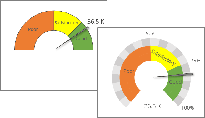
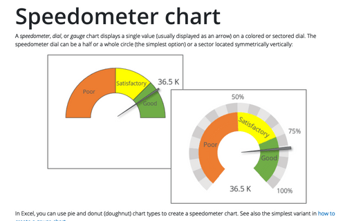
In Excel, you can use pie and donut (doughnut) chart types to create a speedometer chart. See also the simplest variant in how to create a gauge chart.

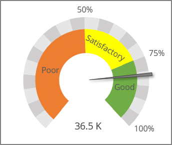
To create a speedometer chart like the one above, do the following:

Prepare data ranges

   1.   To create a speedometer graph, you need several different data ranges:

• The actual or current value:

  For example:

  • Cell B2 contains the actual value that is displayed as an arrow,
  • Cell C2 contains the total amount and the Goal value.
• To display an arrow, calculate the following data:
  
  • Cell A5 contains the current or actual value minus half of the data used for the arrow if you prefer to display a glancing arrow:

    = <value> - <arrow> / 2

  • Cell A6 contains the data used to display an arrow:
    • 1 if you have small amounts or it is enough to display an arrow as a simple line,
    • 1% of the Goal value if you prefer to see a glancing arrow:

      = <Goal> * 1%

  • Cell A7 contains the residual value:

    = <Goal> - SUM (A5:A6) or = <Goal> - <value> - <arrow> / 2

  • Cell A8 contains the value for the invisible section of the chart:
    • The value is equal to the Goal value to display the exactly half-cycled speedometer chart like in the first example:

      = <Goal>

    • Any other value, for example, 30% of the Goal value like in the second example:

      = <Goal> * 30%

• The qualitative ranges are displayed as colored zones:

  For example, using the  poor ,  satisfactory , and  good  value ranges, which are distributed as follows:

  

  The empty value is an invisible value that corresponds to the value in cell A8:

  • 100% for the first example,
  • 30% for the second example.

Create a combo chart

   2.   Select the data (in this example, A5:A8, E4:E8).

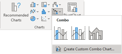
   3.   On the Insert tab, in the Charts group, click the Combo button, then choose Create Custom Combo Chart...:

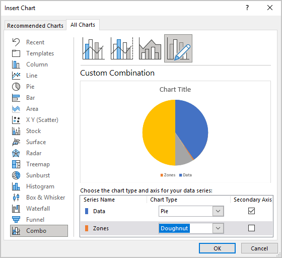
In the Insert Chart dialog box:

• For the data series with values (in this example, series Data):
  • Choose the Pie chart type,
  • Ensure that the Secondary axis checkbox is selected.
• For the second data series with zones (in this example, series Zones), choose the Doughnut chart type:

Format chart

   4.   Optionally, remove the chart title and the legend.

Select the Pie data series

   5.   Select the Pie data series (in this example, series Data) by doing one of the following:

• Select the chart, then on the Chart Format tab, in the Current Selection group, from the Chart Elements list, select the appropriate data series:
  
• Right-click on the chart plot area, then select Format Plot Area... in the popup menu:
  

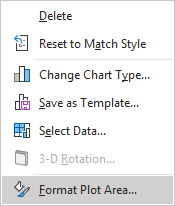
  On the Format Plot Area pane, click the arrow next to Plot Area Options, then choose the element you need from the dropdown list:

  

Rotate the Pie data series

   6.   On the Format Data Series pane, on the Series Options tab, change the Angle of first slice setting to:

• 270^o for the first example:
  
• ~222^o for the second example:

  = (SUM (<Zones>) / 2 + <empty>) / (SUM (<Zones>, <empty>) * 360^o)

Select the Pie data points and format them

   7.   Select the data point of the Pie chart data series by doing one of the following:

• Double-click twice on the data point you want to format,
• Hold the Ctrl key and use the arrow buttons to select your desired chart element.

If needed, right-click on the selection and choose Format Data Point... in the popup menu.

   8.   On the Format Data Point pane, on the Fill & Line tab:

• For the data points but the data point for the arrow (in the example, A6):
  • In the Fill section, select No fill,
  • In the Border section, select No Line:
  
• Choose the appropriate filling for the arrow data point (see more about filling in Microsoft Excel).

For example:

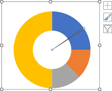
Format the Doughnut data series

   9.   Repeat step 4 to select the Doughnut data series (in this example, series Zones).

   10.   Repeat step 5 to rotate the second data series:

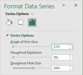
   11.   Repeat step 6 to open the Format Data Point pane for each data point from the Doughnut data series.

On the Format Data Point pane, on the Fill & Line tab:

• Choose the appropriate filling for the data points but the last one (in the example, E8),
• Hide the last data point:
  • In the Fill section, select No fill,
  • In the Border section, select No Line.

For example:

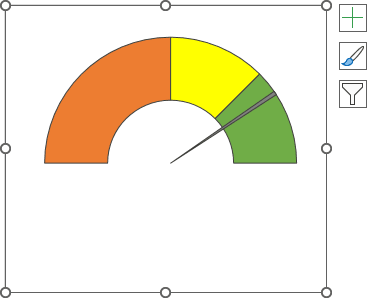
You can then make any other adjustments to get the look you desire.

Notes:

1. To make an arrow a little "bigger" than another data on the chart, select that data point, then on the Format Data Point pane, on the Series Options tab, change the Point Explosion setting to 5%:
   
2. You can add several data series to your chart with the Doughnut chart type:

See also How to create dependent on a volume chart title.