How to hide points on the chart axis

Standard Excel formatting includes a variety of built-in formats that cover general, numeric, currency, percentage, exponential, date, time, and custom numeric formats. You can also design custom formats based on one of the built-in formats. See more about conditional formatting for chart axes.

Using standard formatting, you can also hide certain types of numeric data: positive values, negative values, or zero. Standard formatting of numeric data consists of four parts, separated by a semicolon (or comma, see how to change a semicolon to a comma and vice versa):

{positive value}; {negative value}; {zero}; {text value}

• If you write two formats, the first applies to positive and zero values, and the second applies to negative values,
• If you write three formats, the first applies to positive values, the second to negative values, and the third to zero,
• If you write four formats, they apply to positive, negative, zero, and text values, respectively.

To hide some type of numeric points in the Excel for Microsoft 365 chart axis, do the following:

   1.   Right-click on the axis and choose Format Axis... in the popup menu:

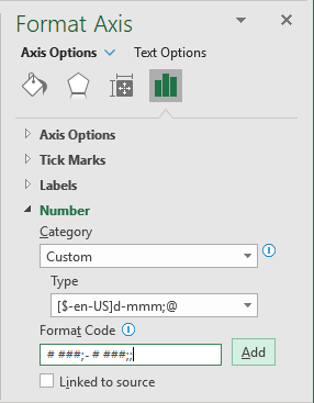
   2.   On the Format Axis task pane, in the Number group, select Custom category and then change the field Format Code:

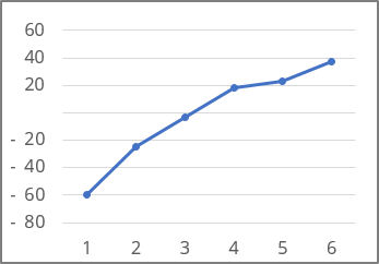
To hide zeros, type # ###; - # ###; ; or # ###; - # ###;

The first applies to positive values, the second to negative, and the third to zero (for more details, see Conditional formatting of chart axes).

   3.   Click the Add button.

Notes:

• To display only positive values, type # ###;:
  
• To hide only negative values, type # ##0; or # ###;;0;:
  
• To display only negative values, type ; - # ###;:
  

See also this tip in French: Comment masquer des points sur l'axe du graphique.