Creating a drop-down list in a cell

Create a drop-down list for the cell

To create your own drop-down list for the cell, do the following:

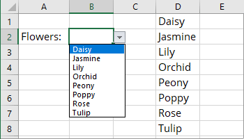
   1.   Create a column or a row of the items in the active spreadsheet for the drop-down list.

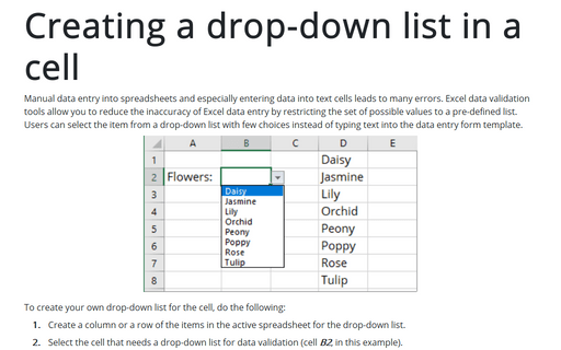
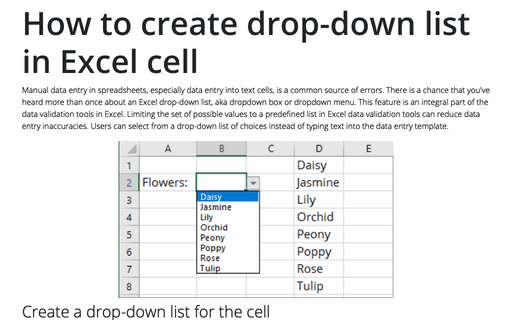
   2.   Select the cell that needs a drop-down list for data validation (cell B2, in this example).

   3.   On the Data tab, in the Data Tools group, click Data Validation:

  or  

   4.   In the Data Validation dialog box, on the Settings tab:

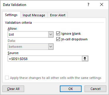
• In the Allow drop-down list, select the List item.
• In the Source box, specify the range that contains the drop-down list items (in this example, the range is D1:D8).
• Check the In-Cell Dropdown option to show the drop-down list. Otherwise, Excel validates your data entry but does not show the drop-down button to select items from the list.

   5.   Click OK.

Notes:

• You can hide the range of values used in the Source box or create it on the protected sheet that you can hide.
• You can add the drop-down list to multiple cells by selecting the appropriate cells or copy/paste the cell with a list.
• If the list is short, you can avoid Step 1. Instead, type your list items (separated by commas) in the Source box in the Data Validation dialog box:
  
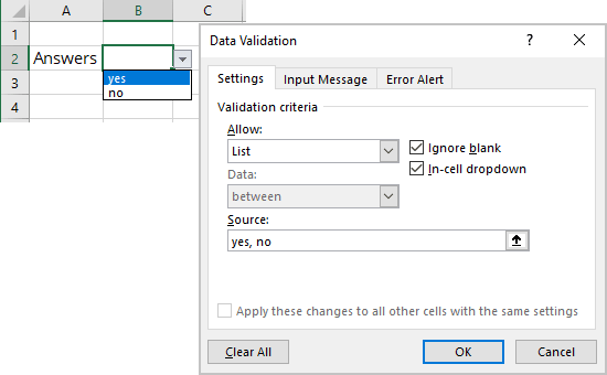
• If you plan to share your workbook with users of Excel 2007 or earlier, make sure that the list is on the same sheet as the drop-down list. Alternatively, you can use a named range.

Remove a drop-down list for the cell

   1.   Select the cell or range of cells with the drop-down list for data validation (cell B2, in this example).

   2.   On the Data tab, in the Data Tools group, click Data Validation:

  or  

   3.   In the Data Validation dialog box, on the Settings tab:

   4.   Click the Clear All button. Check the Apply these changes to all other cells with the same settings check box before clicking the Clear All button if you want to remove all other drop-down lists with similar settings.

See also this tip in French: Création d’une liste déroulante dans une cellule.