Applying Conditional Formatting

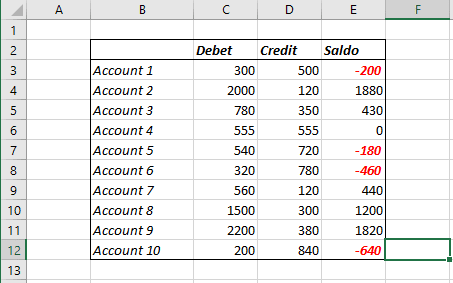
For example, if you wanted to separate all the negative figures:

To apply the conditional formatting, follow these steps:

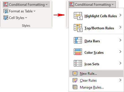
   1.   On the Home tab, in the Styles group, click the Conditional Formatting drop-down list, and then click New Rule...:

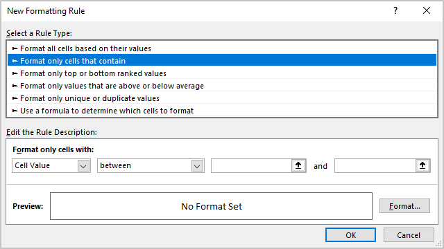
   2.   In the New Formatting Rule dialog box:

• In the Select a Rule Type list, select Format only cells that contain:

• Be sure that Cell Value is selected in the Format only cells with drop-down list on the left of the dialog box.
• In the next drop-down list to the right, select the condition.

  The default is Between. Other conditions include Equal To, Greater Than, Less Than, and other possibilities. Use the drop-down list to select the appropriate condition.

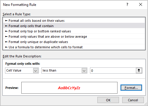
• After selecting the condition, specify a cell, value or formula for the conditional formatting.

  For example, if you select Less Than as the condition, specify a cell in the worksheet that contains a value that can be used for comparison with the cells that you are applying the conditional formatting to.

  If you enter a formula, start it with an equal sign (=).

• Click the Format button in the New Formatting Rule dialog box and select the formatting options for your condition in the Format Cells dialog box. Then click the OK button.

   3.   Click the OK button to close the New Formatting Rule dialog box.

You are returned to the worksheet. Cells that meet the condition you set up for conditional formatting will be formatted with the options you specified.

See also this tip in French: Comment utiliser la mise en forme conditionnelle.