Show chart data in hidden cells

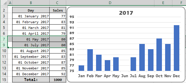
For example, there is some hidden data in the table:

If you want to see hidden data in the chart, do the following:

   1.   Select the chart data by doing one of the following:

• Under Chart Tools, on the Design tab, in the Data group, choose Select Data:
  
• Right-click in the chart area and choose Select Data... in the popup menu:
  

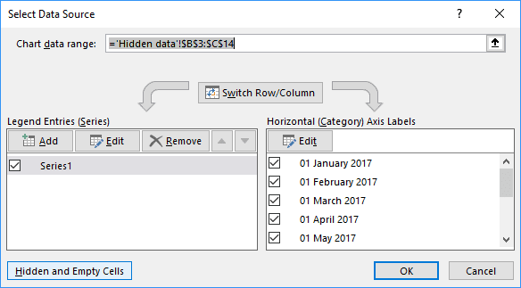
   2.   On the Select Data Source dialog box, click the Hidden and Empty Cells button:

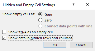
   3.   On the Hidden and Empty Cell Settings dialog box, check the Show data in hidden rows and columns checkbox:

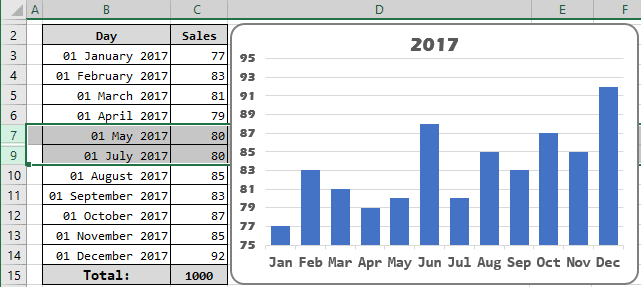
Excel will show all hidden data on your chart:

See also this tip in French: Afficher les données du graphique dans les cellules masquées.