How to sum cells by criteria
Excel
2016
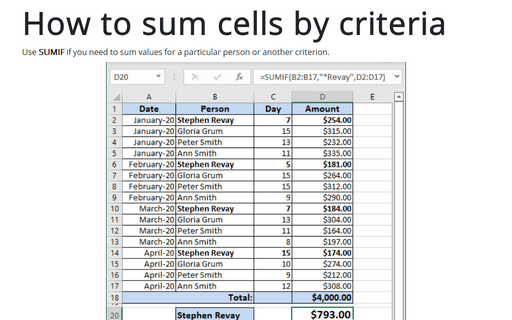
Use SUMIF if you need to sum values for a particular person or another criterion.
To sum cells by criteria, do the following:
1. Select the cell that will contain the result.

2. Do one of the following:
- On the Formula tab, in the Function Library group, select the
Math & Trig button:

Choose SUMIF in the list.
- Click the Insert Function button
 in the left of the Formula bar:

In the Insert Function dialog box:

- select Math & Trig in the Or select a category drop-down list,
- select SUMIF in the Select a function list.
3. In the Function Arguments dialog box:
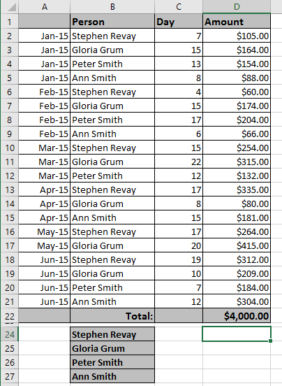
- The Range field determines the range of cells Excel will look to perform the count in. In this example, the cell range is B2:B21.
- The Criteria is a conditional statement that is similar to the conditional statement in the IF statement.
- The Sum_range field tells Excel which cells to add when the criteria are met for each cell in the range. In this example, the cell range is D2:D21.
4. Press OK.
Notes:
- You can enter this formula using the keyboard, for this example:
= SUMIF (B2:B21, "*Revay", D2:D21) - You can use the wildcard characters, question mark (?), the asterisk (*) in the criteria. A question
mark matches any single character; an asterisk matches any sequence of characters. If you want to
find an actual question mark or asterisk, type a tilde (~) before the character. For example:

- Microsoft Excel provides additional functions that can be used to analyze your data based on a
condition or criteria:
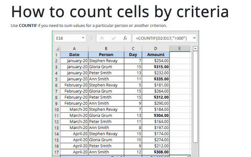
- To count the number of occurrences of a string of text or a number within a range of cells, use the COUNTIF function (see How to count cells by criteria for more details).
- To have a formula return one of two values based on a condition, use the IF function.
- To analyze data in a list based on criteria, such as profit margins or product types, use the database and list management functions (DCOUNT, DCOUNTA, DSUM, etc.).
See also this tip in French: Comment calculer la somme des cellules par critères.

