Custom cell format

To define a custom format, follow these steps:

   1.    Enter sample text for the format in a cell, and then select that cell (Excel then displays the sample text in the new format, which helps to see the effects of your changes).

   2.    Do one of the following:

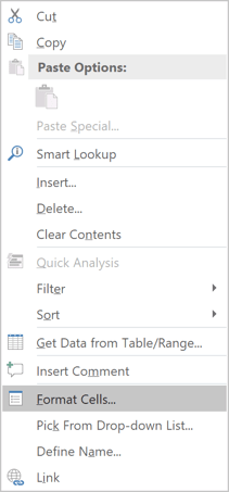
• Right-click on the selection and choose Format Cells... in the popup menu:
  
• On the Home tab, in the Number group, click the dialog box launcher:
  

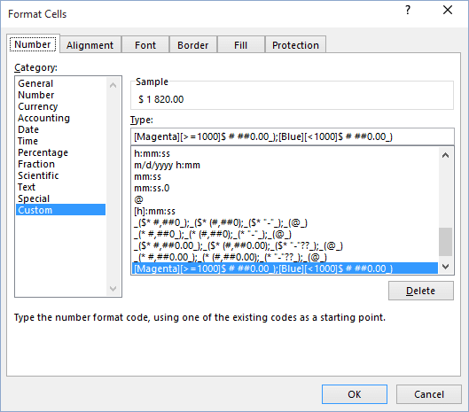
   3.    On the Number tab, in the Category box, select the Custom item.

   4.    In the Type list box, select the custom format on which you want to base your new custom format. Excel displays the details for the type in the Type text box.

   5.    If the details for the type extend beyond the Type text box, double-click in the Type text box to select all of its contents, issue a Copy command (for example, press Ctrl+C), and then paste the copied text into a text editor, such as Notepad. (For a shorter type, you can work effectively in the Type text box. For a longer type, it's easier to have enough space to see the whole type at once.)

   6.    Enter the details for the four parts of the type, separating the parts from each other with a semicolon.

• If you write two formats, the first applies to positive and zero values, and the second applies to negative values.
• If you write three formats, the first applies to positive values, the second to negative values, and the third to zero.
• If you write four formats, they apply to positive, negative, zero, and text values, respectively.

   7.    If you're working in a text editor, copy what you typed and paste it into the Type text box. Check the sample text to make sure it seems to be correct.

   8.    Click the OK button.

See also this tip in French: Format de cellule personnalisé.