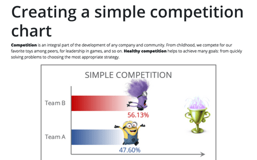
Creating a simple competition chart

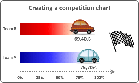
To create the chart like this one, do the following:

   1.   Select all necessary data - in this example, C4:D4, C17:D17:

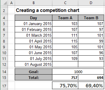
   2.   On the Insert tab, in the Charts group, click the Bar button:

Choose the Clustered Bar chart.

   3.   Right-click on the chart and in the popup menu, select Add Data Labels and again Add Data Labels:

   4.   Select one of the data labels:

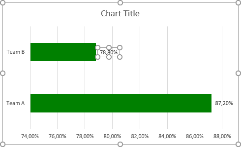
   5.   Right-click on the selected data label and select Format Data Label... in the popup menu:

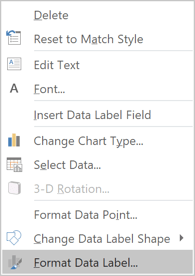
   6.   On the Format Data Label pane, on the Fill & Line tab, in the Fill group, check Picture or texture fill and then click on the File... button (if you have the picture already), Clipboard or Online... (if you would like to upload picture from Internet):

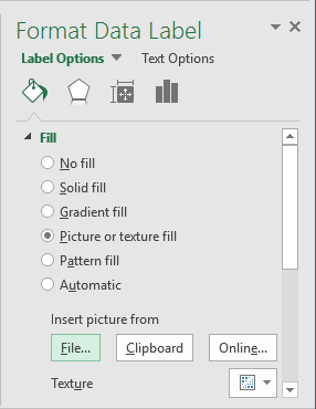
   7.   Make changes for the second data label (repeat steps 4 -6 for it).

Make any other adjustments to get the look you desire, see also Creating a chart with dynamic labels.

See also this tip in French: Créer un graphique de compétition simple.