How to change number, currency, or accounting format

You won't find the Excel settings for each used format, as Excel uses the format configured in the operational system (Windows 10).

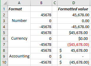
According to the U.S. standards, the Currency format and the Accounting format can be used to display monetary values:

• In the Currency format, the currency symbol appears right next to the first digit in the cell, and the decimal points appear aligned in the column
• In the Accounting format:
  • The currency symbol and the decimal points appear aligned in the column,
  • Zeros are indicated by a hyphen,
  • Negative numbers are indicated in brackets:

Automatic number formatting

When you type a value in a cell, Excel can automatically apply a predefined number format to a cell:

• If a number contains commas, Excel applies comma formatting to separate thousands (such as 123,456,789).
• If a number contains a percent symbol (%), it may be converted to a percentage format.

  Note: See below how to change the way to apply the percentage format in Excel.

• If a number contains a slash (/), it may be converted to a date or fraction format.
• If a number contains a hyphen (-), it may be converted to a date format.
• If a number contains a colon (:) or is followed by a space and the uppercase or lowercase letter A or P, it may be converted to a time format.
• If a number contains the letter E (uppercase or lowercase), it may be converted to scientific notation, also known as the exponential format.

Change format

To change the format for the selected cell or cells, do the following:

• Using the keyboard:

• On the Home tab, in the Number group, open the Number Format dropdown list:
  

  From the Number Formats dropdown list:

  

  Choose the format you need, see How to change number cells format easily for more details.

• Do one of the following:
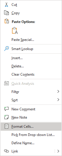
  • Right-click on the selection and choose Format Cells... in the popup menu:
    
  • On the Home tab, in the Number group, click the dialog box launcher:
    
  • Press Ctrl+1.

  In the Format Cells dialog box, on the Number tab, in the Category list, choose the format you need:

  

• Using the mouse: Number-Formatting Keyboard Shortcuts

  Key Combination	Formatting Applied
  Ctrl+Shift+$	Currency format with two decimal places (negative numbers appear in parentheses) – see how to change the currency format
  Ctrl+Shift+^	Scientific notation number format, with two decimal places
  Ctrl+Shift+!	Two decimal places, thousands separator, and a hyphen for negative values

See How to change number cells format easily for more details.

Note: If a cell displays a series of hashes such as #########, this usually means that the column width is not wide enough to display the value in the selected number format. To display the value correctly, change the column width (see How to change width of gridlines in Excel) or change the number format.

Change currency symbol

To change the currency symbol, do one of the following:

• On the Home tab, in the Number group, click the Accounting Number Format button:

  From the Accounting Number Format dropdown list:

  • Choose the format you prefer:
    
  • Click More Accounting Formats... to open the Format Cells dialog box.
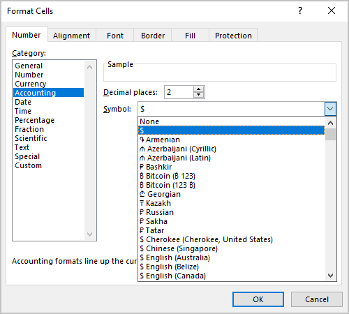
• Click Ctrl+1, then in the Format Cells dialog box, choose the appropriate currency symbol from the Symbol dropdown list:

See how to change the currency symbol used by default.

Two ways to apply the percentage format

There are two ways how Excel can convert the entered number with a percent sign, entered in a cell formatted as a percentage, to a percentage format:

• Without any changes (by default). For example, enter 12 to display 12.00% or enter .12 to display 0.12%.
• Using decimal format. For example, enter 12 to display 1200%, or enter .12 to display 12.00%.

To change the option for percentage format, do the following:

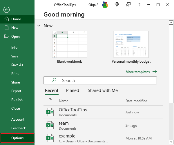
   1.   On the File tab, click the Options button:

   2.   On the Advanced tab, under Editing options, select or deselect the Enable automatic percent entry checkbox:

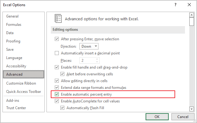
• If the Enable automatic percent entry checkbox is selected (used by default), the entered normal value will be displayed as a percent.
• If the Enable automatic percent entry check box isn't selected, you need to enter the value as a decimal to be displayed as a percent.

Numeric limitations in Excel

Excel allows numbers up to 15 digits. For example, if you enter a large value such as 123,456,789,123,456,789 (18 digits), Excel will store it with only 15 digits. So, this 18-digit number it displays as 123,456,789,123,456,000.

To store large numbers, such as credit card numbers, which are usually 16 digits long, use the text format:

• The easiest way is to format the cell as text. To format the selected cell or cells, do one of the following:
  • On the Home tab, in the Number group, open the Number Format dropdown list, then choose Text:
    
  • Click Ctrl+1 to open the Format Cells dialog box and choose Text from the Category list:
    
• Put an apostrophe (') before the number:

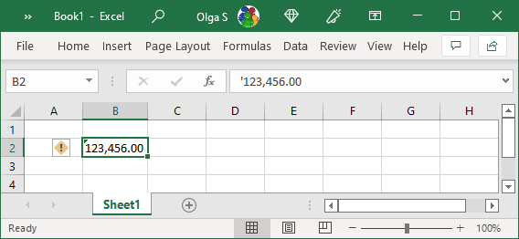
Both methods will force Excel to interpret the cell value as text instead of a number.

Here are some of the other numeric limits:

• The largest positive number is 9.9E+307
• The smallest negative number is -9.9E+307
• The smallest positive number is 1E–307
• The largest negative number is –1E–307

All these numbers have only 15 digits of precisions.

See also How to avoid misleading numbers.